Algebraic Analysis notes Lecture 5 (16 Jan 2019)

Notes for Lecture 4

Last time: Hard Lefschetz gives an orthogonal decomposition $H^k(X, \mathbb C) = \bigoplus_{2r \leq k}^\bot \eta^r H_{prim}^{k-2r} (X; \mathbb C)$ with respect to a Hermitian form on $H^k (X, \mathbb C)$ defined using the Poincare pairing.

On the other hand, Hodge theory gives a decomposition $H^k (X; \mathbb C) = \bigoplus_{p+q = k}^\bot H^{p,q} (X)$ . So $H^k (X; \mathbb C)$ has an orthogonal decomposition into pieces coming from $H^{p,q}_{prim} = H^k_{prim} (X; \mathbb C) \cap H^{p,q} (X)$ .

Hodge-Riemann bilinear relations: The form $(-1)^{\frac{k(k+1)}{2}} i^{p-q} \mathbb H_k$ is positive definite on $H^{p,q}_{prim}$ .

Products: Fundamental group (or higher homotopy groups) we have $\pi_1 (X \times Y) \cong \pi_1(X) \times \pi_1(Y)$ . (Co)homology is harder.

Kunneth Formula: for k a field, $H^* (X \times Y; k) \cong H^*(X; k) \otimes H^*(Y; k)$ .

Locally products: A fibre bundle consists of a total space E, a base space B, a fibre F, and a map $p \colon E \rightarrow B$ , such that for any point x in the base B, there is a neighborhood U of x and a homeomorphism such that the following diagram commutes

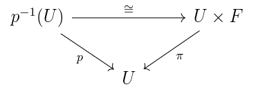
Question: what is the relationship between $H^*(E)$ and $H^*(B)$ and $H^* (F)$ ?

Example: $S^3$ is fibred over $S^2$ with fibre $S^1$ . Think of $S^3$ as $\{(z_0, z_1) \in \mathbb C^2 \mid |z_0|^2 + |z_1|^2 = 1\}$ and $S^2 = \mathbb C \cup \{ \infty \}$ . Define a map $S^3 \to S^2$ by $(z_0, z_1) \mapsto z_0/z_1$ . This is called the Hopf fibration.

$H^*(S^1) = \mathbb Z, \mathbb Z, 0, 0, \dots$
$H^*(S^2) = \mathbb Z, 0, \mathbb Z, 0, \dots$
$H^*(S^3) = \mathbb Z, 0, 0, \mathbb Z, \dots$

Then we can draw $H^p (S^2) \otimes H^q (S^1)$ in a grid, spectral sequence

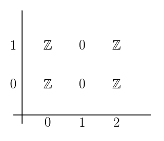
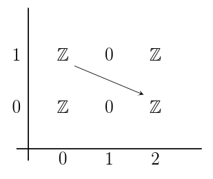
If we take sums along diagonals, i.e. $\bigoplus_{p+q=i} H^p(S^2) \otimes H^q(S^1)$ , we get $\mathbb Z, \mathbb Z, \mathbb Z, \mathbb Z, 0, \dots$ , but this isn’t exactly the same as $H^*(S^3)$ .

Answer [Leray-Serre]: If B is simply-connected, then there is a spectral sequence $E_2^{p,q} = H^p (B; k) \otimes H^q (F; k) \Rightarrow E_\infty^{p+q} = H^{p+q} (E; k)$ .

Roughly, $H^*(E)$ is built out of $H^*(B) \otimes H^*(F)$ “after some cancellations”. The differential cancels out $\mathbb Z$ s on the next page of the spectral sequence:

the arrow indicates the differential, which cancels out those copies of Z

Theorem [Deligne-Blanchard]: Let $f \colon E \to B$ be a family of smooth projective varieties. Then the Leray-Serre spectral sequence degenerates at $E_2$ ! There is no cancellation. (Thanks to Daniel Litt for pointing out on Twitter that this is only true for cohomology with coefficients in a field of characteristic 0!)

So $H^i (E) \cong \bigoplus_{p+q = i} H^p(B) \otimes H^q (F)$ for B simply-connected.

The theory of intersection cohomology and perverse sheaves gives a way to simultaneously generalize all of this! Poincare duality, weak & hard Lefschetz, and Hodge-Riemann bilinear relations, intersection cohomology will tell us that some modification of these theorems hold for any projective algebraic variety (not necessarily smooth), and a vast generalization of Deligne’s theorem to arbitrary proper algebraic maps $f \colon X \to Y$ .

To do this we’ll need the theory of sheaves and homological algebra and category theory!

Presheaves

Let X be a topological space. Let Op(X) denote the category with open sets of X for objects and inclusions for morphisms. For a ring k, a presheaf of k-modules on X is a functor $F \colon Op(X)^{op} \to k-mod$ . A morphism of presheaves $f \colon F \to G$ is a natural transformation. We write PreSh(X; k) for the category of presheaves.

Let’s unpack this definition. F is a rule which assigns to each open subset U of X a k-module F(U), and to each inclusion $U \subseteq V$ a homomorphism of k-modules $res_{U,V} \colon F(V) \to F(U)$ , called “restriction”. $\alpha \in F(U)$ is called a section of F over U. Notice that functoriality gives $res_{U,U} = id_{F(U)}$ , and if $U \subseteq V \subseteq W$ then $res_{W,U} = res_{V,U} \circ res_{W,V}$ .

A morphism $f \colon F \to G$ is a collection of k-module homomorphisms $f_U \colon F(U) \to G(U)$ for each U open in X, such that if U is a subset of V, then the following commutes:

I used superscripts to distinguish the two restriction maps, but I don’t know if this is standard

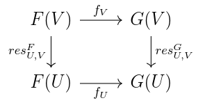
If s is an element of F(V), and U is a subset of V, sometimes we write $res_{U,V} (s) = s|_U$ .

Example: Let M be a k-module. The constant presheaf on X with value M, denoted $\underline{M}_{pre}$ or $\underline{M}_{pre, X}$ , is given by $\underline{M}_{pre}(U) = M$ for all U open in X, and $res_{U,V} = id_M$ for all inclusions $U \subset V$ .