Combinatorics, Lecture 3 (3 Oct 2019)

Lecture 2 here. Thanks again to Tim Hosgood for the beautiful pictures.

The category of species

Last time, we looked at the relationship between species and their generating functions, a formal power series associated to a species which lets you count structures described by the species. Now we’ll take a closer look at species themselves. In particular, there is a category where the objects are species. As is the case in so many branches of math, looking at the category of our main objects of study will be a useful perspective.

There is a category of species, called $\mathsf{Set}^\mathsf{S}$ , with species $G\colon\mathsf{S}\to\mathsf{Set}$ as objects and natural transformations $\alpha \colon G \Rightarrow G'$ as morphisms.

There is a subcategory of $\mathsf{Set}^\mathsf{S}$ where the objects are finite species, denoted $\mathsf{F}^\mathsf{S}$ .

We’ve talked about functors in this class before, but not yet natural transformations. Recall: given categories $\mathcal{C}$ and $\mathcal{D}$ , a functor $G \colon \mathcal{C} \to \mathcal{D}$ sends objects $c \in \mathcal{C}$ to objects $G(c) \in \mathcal{D}$ , and morphisms $f \colon c\to c'$ in $\mathcal{C}$ to morphisms $G(f) \colon G(c) \to G(c')$ in $\mathcal{D}$ such that $G(g \circ f) = G(g) \circ G(f)$ and $G(1_c) = 1_{G(c)}$ .

If $G,H \colon \mathcal{C} \to \mathcal{D}$ are functors, then a natural transformation $\alpha \colon G \Rightarrow H$ assigns to each object $c \in \mathcal{C}$ a morphism $\alpha_c \colon G(c) \to H(c)$ in $\mathcal{D}$ , such that the naturality square

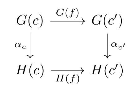
commutes. If all the components $\alpha_c$ are invertible, then we say that $\alpha$ is a natural isomorphism.

Proposition: If $\alpha$ is a natural isomorphism then there exists a natural transformation $\alpha^{-1}$ given by $(\alpha^{-1})_c=(\alpha_c)^{-1}$ .

Theorem: If $\mathcal{C}$ and $\mathcal{D}$ are categories then there is a category $\mathcal{D}^\mathcal{C}$ whose objects are functors $\mathcal{C}\to\mathcal{D}$ and whose morphisms are natural transformations, with composition $\beta\circ\alpha\colon G\Rightarrow J$ of $\alpha\colon G\Rightarrow H$ and $\beta \colon H \Rightarrow J$ given by $(\beta \circ \alpha)_c = \beta_c \circ \alpha_c$ .

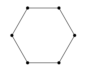
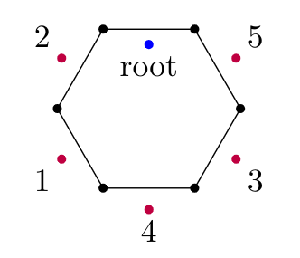
Example: Let $P\colon\mathsf{S}\to\mathsf{F}$ be defined as follows. For a finite set X, let P(X) be the set of all ways of performing the following procedure:

draw a regular (|X|+1)-gon;
label all but one of the sides with the elements of X;
triangulate the polygon.

For example, here is an element of P(5):

Example: Let $B : \mathsf{S} \to \mathsf{F}$ be the species defined as follows: for a finite set X, B(X) is the set of binary, planar, rooted trees whose leaves are equipped with a bijection to X, or X-labelled trees for short. For X=5, B(5) has an element like this:

Theorem: $P \cong B$ , i.e.\ the functors are naturally isomorphic

Proof idea: We need bijections $\alpha_X : P(X) \xrightarrow{\sim} B(X)$ for $X \in \mathsf{S}$ which are natural.

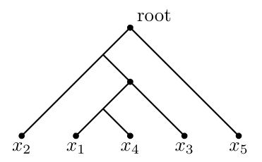
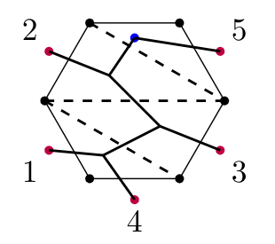
Given the tree in $B(5)$ from the above example, let’s construct the corresponding element of $P(5)$ . We start with a (5+1)-gon.

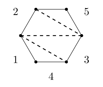
Rather than labelling sides, we’re going to label vertices that we place just outside of each side of the polygon (except for one that we place inside). So we draw $5+1$ vertices, label the top-most one `root’, and the others in the same order as the leaves of our element of $B(5)$ .

Then we draw a copy of our tree inside the polygon.

Finally, we triangulate our polygon by crossing each branch of the tree exactly once.

Theorem: Let $G, H : \mathsf{S} \to \mathsf{F}$ be finite species. If $G \cong H$ then $|G| = |H|$ .

Note that the converse is not true! In future lectures, we’ll look at examples of non-isomorphic species with the same generating functions.

Proof: If there’s a natural isomorphism $\alpha : G \Rightarrow H$ , then there’s a bijection $\alpha_x : G(X) \xrightarrow{\sim} H(X)$ for all $X \in \mathsf{S}$ , so $|G(X)| = |H(X)|$ for all X, thus